CNN classifier for spectrograms with 97.2% acc

#audio-to-image#CustomCNN#human-in-the-loop | June 2026

Introduction

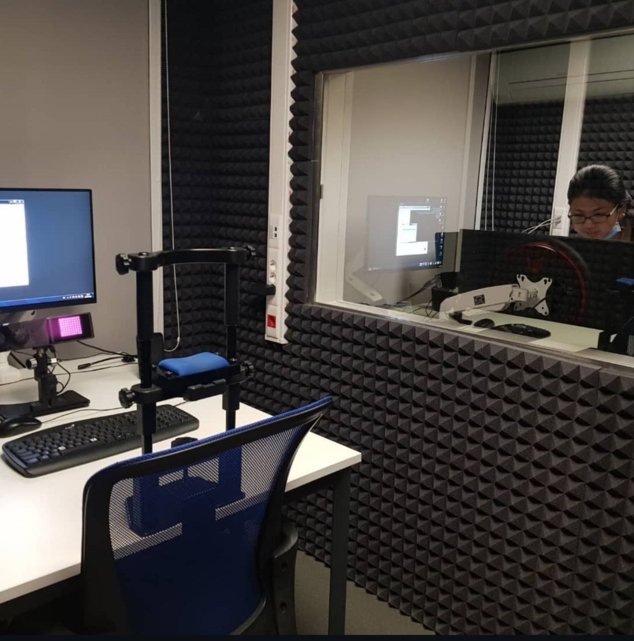
Back in 2024, I conducted an experiment on human attention and language processing. The procedure was quite simple: Participants saw some stimuli on the screen and responded out loud with either PA or TA. Their responses were recorded through a microphone. The hypothesis was that the shift of attention induced by the processing of visual stimuli would affect pitch, latency, and other sound parameters.

The collected dataset consisted of 54 participants, 160 recordings per each = 8640 audio files.

To run any of the actual statistics, every one of those recordings needed a label first: What exactly did the participant say, PA or TA?

The standard way to label recordings in academia is only the manual one: You ask a student to sit with headphones and an Excel sheet, and go through each recording one at a time. It works, of course. But processing 8640 files is quite long and tedious. People get careless somewhere in the middle of the process and are also prone to errors.

Moreover, human hearing is imperfect and not always capable of accurately distinguishing phonemes. It may surprise some readers, but even with sounds as clearly distinct as [p] and [t], one sometimes seems to hear a completely new consonant that combines features of both sounds.

It was precisely this problem that attracted my attention. I thought that there had to be a more reliable (and ideally automated) way to check the records and assign the appropriate label to each of them. Why not try a classification approach in machine learning? There are so many models nowadays that are trained to successfully recognize and classify sound parameters. Or maybe even to build one myself, practicing core NN skills…

With this in mind, I launched this project on the automatic sound classification (spoiler: it ultimately boiled down to image classification), which I named Pa-Ta - after the two-syllable sounds produced by the participants. As we shall see, these sounds were far trickier than they appeared at first glance…

P.S. I did not work on a real deep learning project before this (most of what I knew was from courses and tutorials). So back in 2024, this became my first attempt at building something end-to-end.

What follows in this article is the reasoning I brought in as a scientist and the decisions I made as an engineer.

Understanding the data

Before you start working with the code, you need to ask yourself the fundamental question: what exactly am I dealing with, and what constraints does this impose on my subsequent actions and decisions?

Data structure

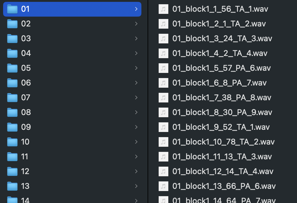
Each participant's response was saved as its own .wav file. 160 files per participant, 54 participants = 8640 files total. That 160 breaks down as 2 experimental blocks * 80 trials each. The files sit in the following layout: a main folder >> one subfolder per participant (e.g., "01") >> that participant's 160 recordings. No files were missing for any participant.

The filenames themselves carry a lot of information, e.g., "01_block1_1_56_TA_1":

• 01 – participant number
• block1 – experimental block (1 or 2)
• 1 – the trial's designed presentation order (out of 80 per block)
• 56 – the trial's actual presentation order (out of 80 per block)
• TA – the response expected by the experiment design
• 1 – the stimuli the participant saw on screen for that trial

Data quality issues

Each file is about 190 KB, 16-bit, and exactly 2 seconds long. Before embarking on anything more systematic, I checked a random sample of files to get an idea of ​​exactly what I was dealing with.

A few things my investigation revealed:

• Most recordings were, as expected, a clean single syllable PA or TA.
• The "correct" label included in the filename wasn't reliable, since participants said the wrong syllable fairly often. Here: the name of the file is "12_block1_11_62_PA_3", but the actual response is TA.
• Some sounds were cut, meaning that the participant srarted to response late.
• Some files were conceptually “empty”, meaning that the participant was silent during the trial, and the mic recorded nothing.
• Some conceptually "silent" files weren't physically silent, meaning that they had a loud cough, breathing, or other noise instead of speech.
• Some recordings contain noise + a speech sound.
• Some files had both syllables (PA-TA or TA-PA) if the participant started answering and then changed their mind mid-response.
• The hardest case is that some recordings sat somewhere between PA and TA. These files are so ambiguous that even a trained ear struggles to recognize the sound. This is where I would not trust a student's or my own judgment.

One participant, 09, misunderstood the instructions. They were pronouncing P and A (or T and A) as two separate sounds instead of one syllable. The data of this participant was removed.

Therefore, the final dataset consisted of 8640 - 160 = 8480 files.

Reframing audio as a CV problem

Why not speech models?

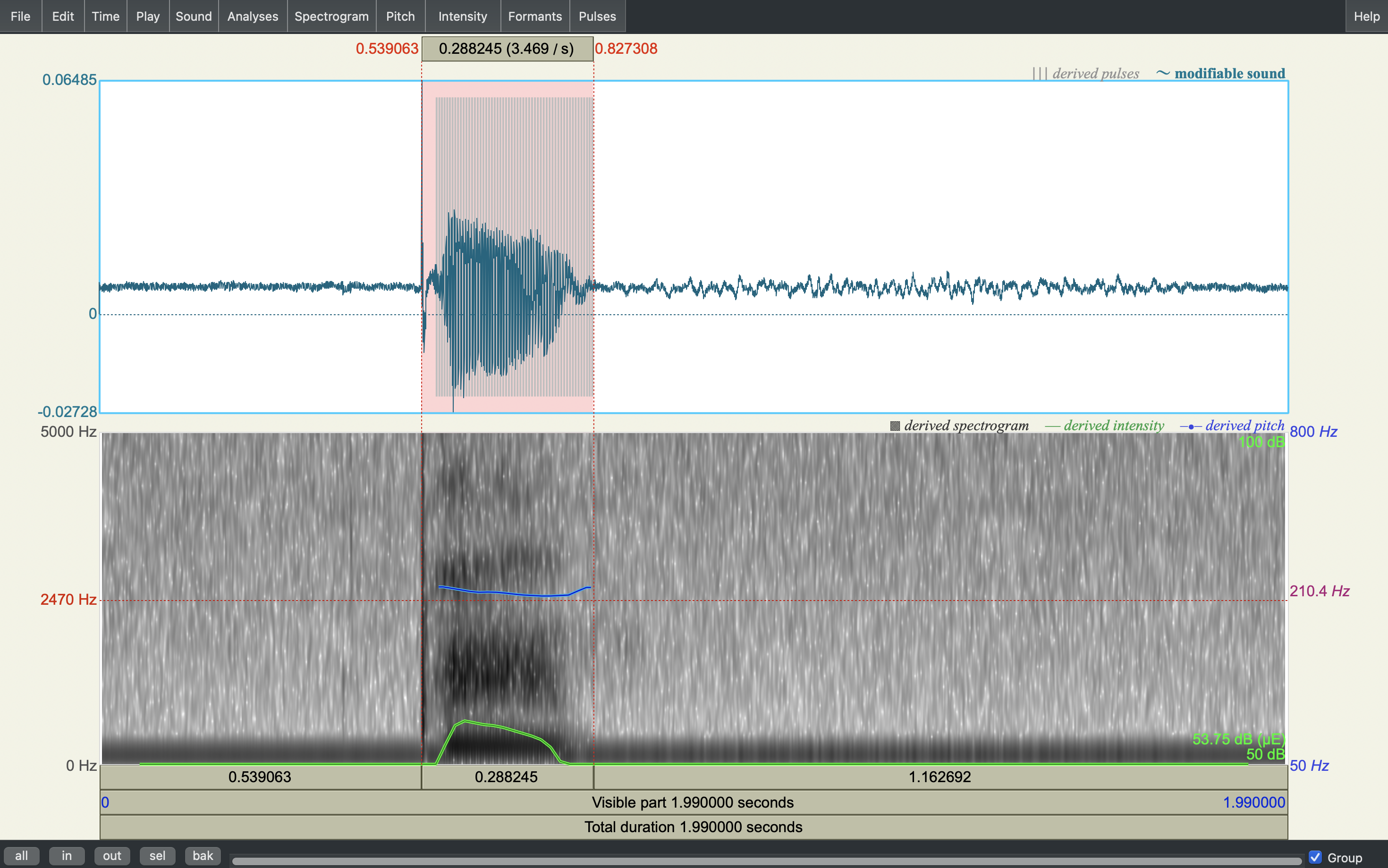
My first idea was to feed the sounds into standard pre-trained speech recognition models (e.g., Whisper). But this approach didn't work since these models are built and trained mostly around words and phrases. PA/TA sounds I needed to classify are much shorter, we are talking ~ 300 ms. The burst spectrum within them is even shorter – from 10 ms. So standard models for recognition of "hello"/"turn left" are not really good at the distinction of patterns hidden in a single syllable.

What pointed me toward a different approach was Praat, the popular old program many psycholinguists use for sound analysis. When they use Praat, they don’t really work with audio as a signal you listen to. Instead, they convert that audio into an image (waveform, spectrogram, etc) and then analyse patterns of that image. The point is that for the human, it is easier to see and extract the relevant features from the image because you can actually observe all the patterns at once. For the computer programs, it does not matter at all because audio and images both eventually reduce to numbers

That was the point where I stopped thinking of PA-TA as a speech recognition task and started thinking of it as an image classification task in the computer vision domain.

The linguistics behind pa vs. ta

In order to decide what kind of image to turn the audio into, I had to understand what makes PA and TA different in the first place.

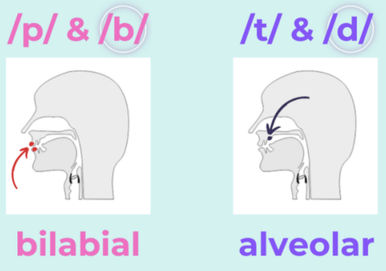
The sounds in human language represent consonants and vowels. The way we build them is by shaping airflow with the tongue, teeth, lips, alveolar ridge, and other organs. In terms of articulation, "pa" and "ta" differ a lot: /p/ is made by closing the lips (bilabial stop), while /t/ is made by connecting the tongue with the alveolar ridge (alveolar stop). These different techniques imply different sound frequencies (how high or low a sound is).

So, we can find differences between "pa" and "ta" in the short noise that bursts at release (burst spectrum), as well as in formant transitions into the following vowel "a".

Namely:

• in the case of PA, the burst has most of its energy in the lower frequencies, and the following vowel starts lower;
• in the case of TA, the burst has more energy in the higher frequencies, and the following vowel starts higher.

Why spectrograms?

The standard way to show frequency and represent how this changes over time is a spectrogram. A spectrogram shows time on the horizontal axis, frequency on the vertical axis (low pitches at the bottom, high pitches at the top), and the strength of the pitch as a color brightness. So, we expect to observe brighter colors appearing lower in the picture in case of PA, and brighter colors appearing higher in the picture in case of TA (spoiler: it is almost not visible for the human eye).

Converting audio to spectrograms

Now, with the physics sorted out, let's actually convert audio files into spectrograms.

First, load the audio file and get its sampling rate with librosa.load(). Next, run a short-time Fourier transform (STFT) via librosa.stft(). In plain terms, this slices the sound into overlapping short-time windows and, for each one, counts frequencies and their strength. The result is a matrix where rows represent frequency bins and columns represent time frames.

The problem is that raw STFT output spans a huge range of amplitude values, so quiet parts and loud parts can't both be seen clearly at once. Let's convert these numbers to decibels with librosa.amplitude_to_db(), compressing that range into something visually readable.

Finally, let's render the matrix as an actual image by using librosa.display.specshow(), RGB. The spectrogram can now be saved as a PNG. Now we have our dataset converted to spectrograms!

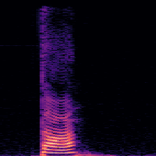
Important details:

• Don't use boundaries, axes, or numbers in the figure. The model has to learn the sound itself, not accompanying artifacts from matplotlib.
• Every image has to be the same pixel size, since that's the input layer's size in the NN. This is controlled by plt.figure(figsize=), but there's a catch. If the underlying audio files vary in length, squashing them all to the same width distorts actual time-frequency features and teaches the model the wrong patterns. Fortunately, this is not a problem in my case since each sound in the dataset is exactly 2 sec long.

Designing the CSV table

The set of images is ready. At this stage, the question remains as to how the tracking is carried out.

An important moment is that this needed to work from two angles at once. On the one hand, the model itself can just read images straight out of structured train/val folders. On the other hand, the scientists want the data as a CSV, with columns like participant number, trial number, presented stimulus, correct (designed response), and actual response – the last is what the model has to predict and fill in. So the CSV had to serve both audiences.

I created a CSV file containing the columns expected by the researchers, and then added a few more required for the model to function (image path, audio path, and label).

Labeling bottleneck

Each audio file needs a label — PA, TA, or N/A (missed/broken/error). However, none of the responses has the label yet. Although we know what each response was supposed to be based on the info encoded in the filename, the earlier data investigation already showed that we can not trust this info: There were too many discrepancies between what was designed and what participants actually said. Meanwhile, the model needs real training data to work with. That said, I have to prepare labels manually.

There are two main questions at this stage: 1) how to create labels efficiently, and 2) how many of them do we need for successful inference.

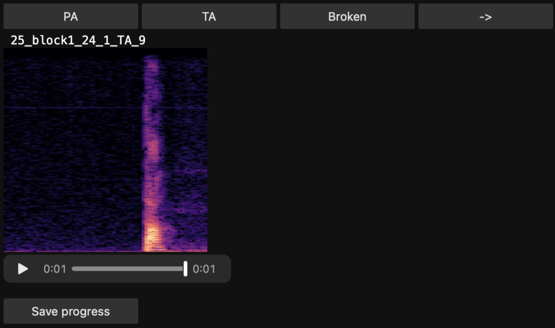
Building a labeling widget

Opening each file one at a time and typing a syllable into a CSV cell is not really time-efficient. Really, it is so crucial that labeling hundreds of files does not turn into a second full-time job! So, I needed something fast, interactive, and convenient.

Let's build an interface for labeling using ipywidgets. The core piece is a widgets.Output() object, because it is like a container for info presentation. When the display is updated, the output is cleaned, and the function set_new_trial() is implemented, setting up a new output. What this function does in detail: it reads the CSV, chooses only rows that have an empty "label" column, takes one random row, and displays the sound alongside its corresponding spectrogram. The random order was important because it allowed for avoiding biasing the initial labeled set toward, say, only the first few participants or one experimental block.

At this point, we can already hear and see a random, unlabeled response. Now, let's create a way to manipulate the widget by building buttons with widgets.Button().

What buttons did I add:

• Next – skip to a new random trial without labeling this one
• PA – write PA to this row's label and move on to the next trial
• TA – write TA to this row's label and move on to the next trial
• Broken – write ERR to this row's label and move on to the next trial
• Save progress – write the CSV to disk and print a running count of how many trials are labeled so far.

Finally, let's wrap these five buttons in a widgets.HBox() so they are organized according to the users' preferences.

Once the widget was running, I was able to create labels relatively easily and fast: 1600 trials in ~6 hours.

How much to label? + Class balance

The second question is: how many examples need to be labeled? There is no single correct number, but the generally accepted rule when splitting a dataset is to allocate about 70-80% for training, with the remainder distributed between the validation and test sets.

I decided to grow the labeled set gradually rather than fix it once and freeze it. So my first target amount of labeled trials was around 1500. I felt like this was enough to train a real first model and see the learning patterns.

The problem that appeared during labeling is the class imbalance: it was only 30 examples per ERR class (error/broken/empty recordings) among 1500 labeled trials for PA and TA. The class imbalance is important because if one class dominates, a model can overfit. That is, not actually learning the difference but leaning toward the majority label. Therefore, at this stage, I decided to drop ERR entirely. Instead, my plan was to check them manually later, at the stage of evaluation, based on the model's confidence threshold.

The first resulting dataset for training contained 1600 trials: PA - 800, TA - 800.

Building the data pipeline

We now have a CSV table with 1,600 labeled examples; each contains the path to an image (a spectrogram on disk) and a label. But how exactly will this data be fed into the model?

PyTorch Dataset class

PyTorch has a Dataset class from torch.utils.data - a classical structure for data loading. What it needs is just our CSV (__init__()) and the total number of labels (__len__()).

Its main task is to load and return a single spectrogram-label pair (__getitem__()).

The loading part:

• given an index, it opens the corresponding spectrogram PNG with PIL;
• converts it into RGB;
• runs torchvision transforms you apply (augmentation + resizing + converting PIL Image (H×W×C, values 0-255) to PyTorch tensor (C×H×W, values 0.0-1.0));
• looks up the integer label;
• returns the pair.

Yes, an important thing is that the model needs string labels turned into integers, so the Dataset class expects a label-to-index mapping in __init__(). Let's make 'pa': 0 and 'ta': 1. And let's keep a label-to-name lookup, so results can be explained back after prediction.

Data augmentation: nuances for spectrograms

The next step in image processing is typically augmentation, which allows the model to encounter a wider variety of data than the original set provides. However, augmentation cannot be applied indiscriminately, as it must take the physical meaning of the data into account. I experimented with standard image processing techniques but quickly realized that a spectrogram is not a photograph and requires a completely different approach.

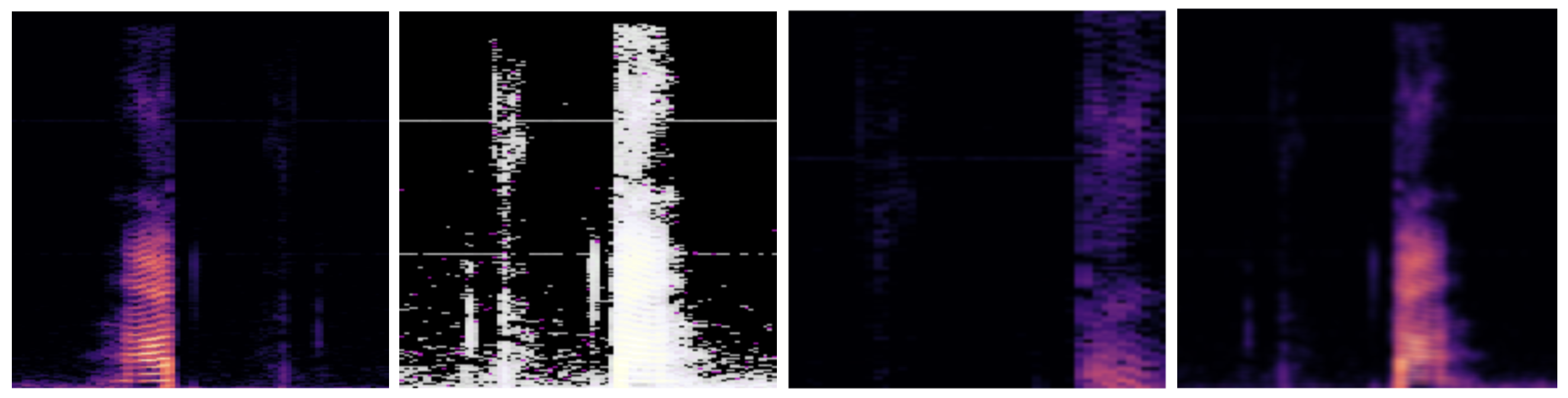
Augmentation methods that do not work with spectrograms:

• Stretching vertically or horizontally, rotation: these change the spectrogram's axes, and the axes stand for real values (time and frequency). Distorting the axes distorts the meaning.
• Flipping: reverses the sound in time, so PA turns into something closer to AP.
• Cropping: a piece of the sound is a different sound, not just a part of an object like in an ordinary photo (say, a cat's ear).
• Gaussian & salt-and-pepper noise / motion blur: corrupt the tiny differences in the burst spectrum that are crucial for classification.
• GridDropout, cutout, random erasing: can hide the burst spectrum and the formant transition into the following vowel. This is the only region we actually care about.
• MixUp and CutMix: blending two sounds, or dropping a patch from one sound into another, just makes a new sound (or a total mess), not a variation of the original one.

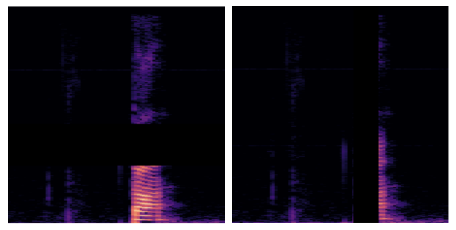
Even the spectrogram-specific augmentations did not seem appropriate:

• Frequency masking: masks random frequency bands (horizontal bars).
• Time masking: masks random time segments (vertical bars).

The reason: these are ultra-short syllables, and the region of interest inside them is even shorter, we are talking a few milliseconds after the sound starts. Different speakers also have different vocal tract shapes and pitch, so the burst's energy doesn't always land in the same frequency band for each person. On top of that, the onset of the sound is highly variable, so there is no fixed position for the region of interest along the time axis either. Because of this, it was noticeably hard to define a fixed range for frequency masking or time masking since it could risk masking out the region of interest.

Theoretically, other options might have worked, but they either made no sense or required linguistic expertise (which was not available to me at the time):

• Grayscale conversion: dropping the color channels, since spectrograms are naturally single-channel anyway. The problem is that it creates exactly the same image, just encoded differently (1 channel vs. 3 channels). Did not make sense.
• Brightness, contrast, hue, saturation: these simulate lighting changes. They do not change time or frequency axes, which is good. But they change the strength of frequencies, like, make everything louder or quieter. It might be a problem and needs an expert validation... E.g., one of the potential problems is that applying the same filter to every image ignores outliers (e.g., a near-whisper response could turn almost black after the transform). There's also a risk of adding frequency patterns that never existed in the real speech (though it needs to be checked with linguists).

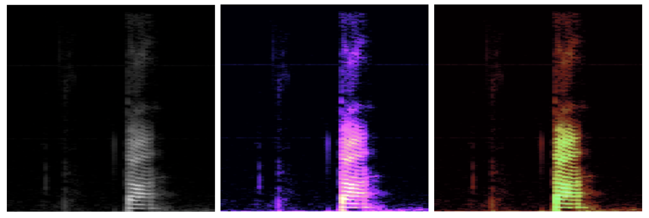
Therefore, none of the augmentations listed above was used in the final pipeline.

Normalization

I standardized pixel values per channel (RGB), using the formula (pixel_value - mean) / std. The mean and standard deviation were calculated across all training spectrograms. Therefore, for this specific domain, the resulting values are centered around zero.

Train/validation split & loaders

The final step before training is splitting the data and building the loaders.

Here, we need to split the data into training and validation sets. If we evaluate the model on the same spectrograms used for training, it is impossible to determine whether it has truly learned the underlying pattern or simply memorized the data. Let us set aside 20% of the data for the validation set and 80% for the training set (ensuring the split is reproducible).

The data split itself must be reproducible. Otherwise, each time the notebook is re-run, training and validation will be performed on slightly different data. Consequently, any changes in accuracy between runs could simply be "noise" caused by the split itself, rather than a genuine improvement.

Also, train and validation sets don't get the same treatment after the split: E.g., augmentation applies only during training, never to validation/test.

Batches (how many trials are processed at once) are shuffled during training but not during validation. Shuffling during training keeps the model from picking up the same ordered files. Without it, the same sequence would repeat every epoch. Validation isn't used to update the model, so shuffling gives nothing there.

That gave 1280 spectrograms for training and 320 for validation, with a batch size of 32. Hooray, the data pipeline is done!

A custom CNN

Design rationale

What model to choose?

I tried fine-tuning pretrained image classification models first (e.g., ResNet50). But it did not work well, because spectrograms are a completely different class of image from, say, photos of a forest or teddy bears (this is what popular pretrained models are trained on). Also, recall that these spectrograms represent ultra-short sounds (average 300 ms), with the region of interest being even shorter (starting from 10 ms).

Because of this (but also mostly because the whole point of this project was to actually learn and practice the CV domain), I decided to build my own custom model from scratch. Since this was my first practical project, it was meant to be just a simple spectrogram model for a 2-class image classification task.

My choice was a Convolutional Neural Network (CNN), with the architecture described below. It is different from, say, a plain fully-connected NN because it does not connect every pixel to every neuron. Instead, it slides filters across the image and looks for local patterns (e.g., edges, blobs, textures). CNN includes many layers: early layers learn simple patterns, while deeper layers combine them into more abstract patterns. Thanks to the convolution, a filter that learned a specific pattern (e.g., a vertical edge) in one part of the image will also catch it elsewhere, without needing to relearn it.

I chose CNN over the alternatives mainly because a plain fully-connected NN is not specifically designed for catching patterns, and also it would need an enormous number of parameters just for the first layer. A Vision Transformer would be an overkill, and due to its heavy structure, it needs a lot more data (1280 training images is not really enough).

I am not saying the architecture below is the best or most effective one for this task. If I approached this project now, I would probably go back to transfer learning, but from a model pretrained on audio spectrograms specifically, like PANNs (Pretrained Audio Neural Networks) or VGGish/YAMNet by Google (although there would be some nuances here as well).

Architecture walkthrough

First, let's import torch.nn that will be needed for the base class nn.Module every model has, and torch.nn.functional for the activation functions.

The full forward pass looks like this (no batch, single image pass):

Input: 3×224×224

Feature extraction

• Conv1 (kernel=3×3, stride=1, padding=1): 32×224×224
• BatchNorm: 32×224×224
• ReLU: 32×224×224
• MaxPool1 (kernel=2×2, stride=2): 32×112×112
• Conv2 (kernel=3×3, stride=1, padding=1): 64×112×112
• BatchNorm: 64×112×112
• ReLU: 64×112×112
• MaxPool2 (kernel=2×2, stride=2): 64×56×56
• Conv3 (kernel=3×3, stride=1, padding=1): 128×56×56
• BatchNorm: 128×56×56
• ReLU: 128×56×56
• MaxPool3 (kernel=2×2, stride=2): 128×28×28
• Conv4 (kernel=3×3, stride=1, padding=1): 256×28×28
• BatchNorm: 256×28×28
• ReLU: 256×28×28
• MaxPool4 (kernel=2×2, stride=2): 256×14×14

Downsampling

• AdaptiveAvgPool: 256×1×1
• Flatten: 256

Classifier head

• Linear1 (+ dropout): 128
• ReLU: 128
• Linear2 (+ dropout): 64
• ReLU: 64
• Linear3 (Output): 2 (logits for PA and TA)

Now let's discuss each part in detail. There will be no math formulas for the forward pass here, because it takes too much space, and the article is already long enough.

Input layer

The transform pipeline resizes every spectrogram to 224×224, and it stays RGB. It means that the input is a tensor of size 3×224×224.

We will start with 4 convolutional blocks. Each block consists of:

Convolution layer

nn.Conv2d() with kernel size = 3, stride = 1, padding = 1

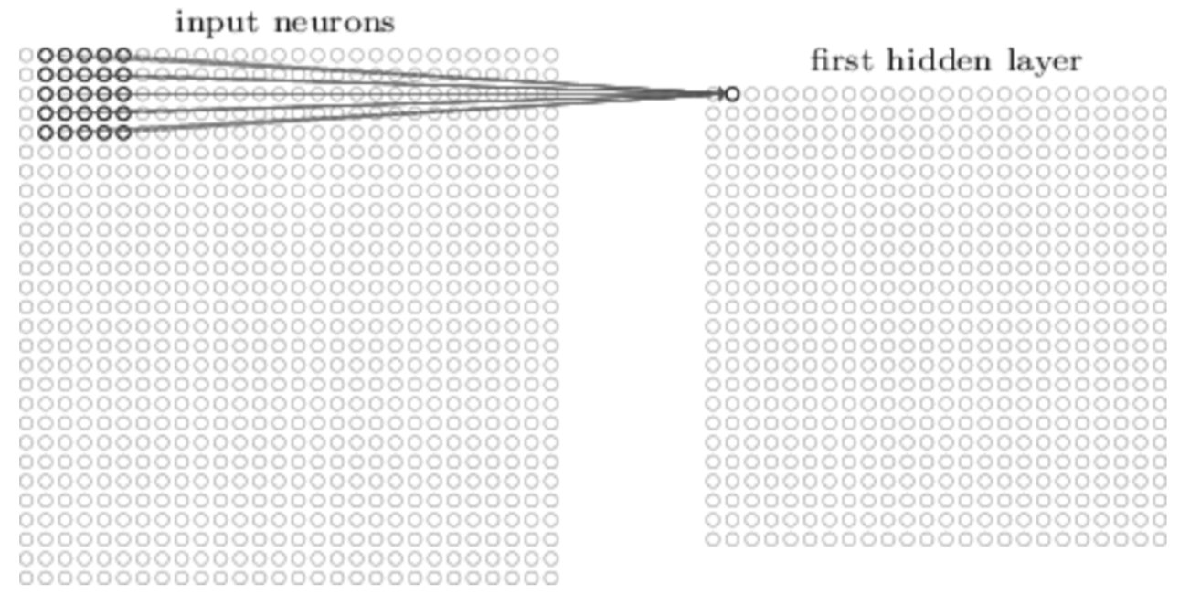
The first hidden layer is connected to the input layer. The kernel (that is, filter) slides across the input layer's neurons, one step at a time. The area covered by the kernel is called a local receptive field for the hidden neuron - a region of the input neurons (a 3×3 grid in our case), where all neurons are connected to that single hidden neuron. For each local receptive field, there is a different hidden neuron in the first hidden layer.

The output produced by applying a filter to an input in CNN is called a feature map. A complete convolutional layer might consist of several different feature maps (by applying several different filters to the input). Within one feature map, the same weights and bias are applied at every local receptive field, meaning all the neurons in that feature map detect exactly the same feature, just at different locations in the input.

Each of the N feature maps is defined by its own separate set of shared weights and a single shared bias. The result is that the network can detect N different kinds of features, with each feature being detectable across the entire image.

Let's grow channels in the first hidden layer from 3 to 32. We will continue the same logic in each of the following convolutional blocks, growing channels to 64, 128, and 256 by the end of the 4th convolutional block.

After applying convolution, the hidden layer size should become smaller than the input layer. But we use padding=1 (adding a one-pixel border of zeros around the image). Therefore, the spatial size doesn't change.

Batch normalization

nn.BatchNorm2d()

Next, let's add a batch normalization layer matched to each conv layer's channel count. Batch normalization takes the outputs of a layer and re-centers and re-scales them, using the statistics of the current mini-batch. So the numbers flowing through the NN stay in a stable and consistent range as training progresses (instead of drifting or exploding).

ReLU

F.relu()

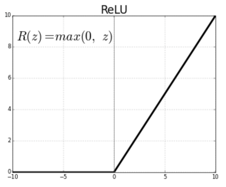
Next is the ReLU activation function. It simply zeroes out any negative value and leaves positive values untouched. We need it to add non-linearity to the model. Without it, stacking many linear regressions would just collapse into one single linear regression (no matter how deep the NN is), and the model would not be able to learn complex non-linear patterns.

Max pooling layer

nn.MaxPool2d() with kernel size = 2, stride = 2

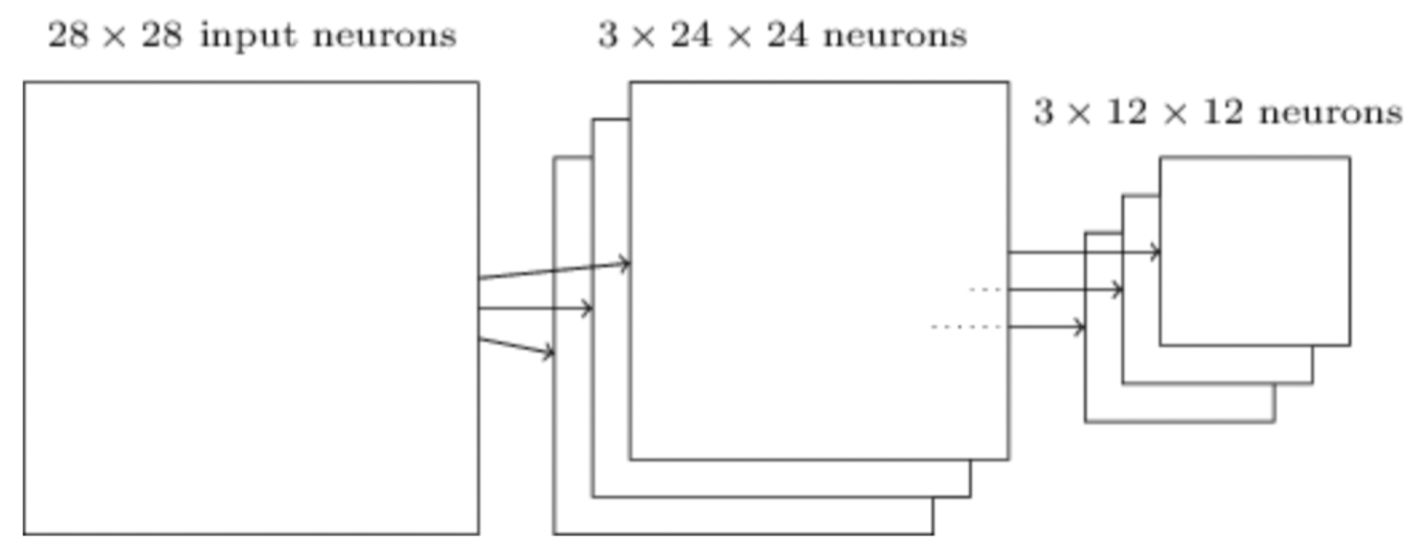
This same layer is reused in every convolutional block as well. It slides a 2×2 kernel across the image and keeps only the largest value in each window (the rest gets discarded). By using this procedure, max pooling shrinks the image by half and keeps only the strongest signal.

In the first convolutional block, it shrinks the image from 224×224 to 112×112. In the following convolutional blocks, the size will change to 56×56, 28×28, and 14×14, respectively.

Adaptive (global) pooling layer

nn.AdaptiveAvgPool2d()

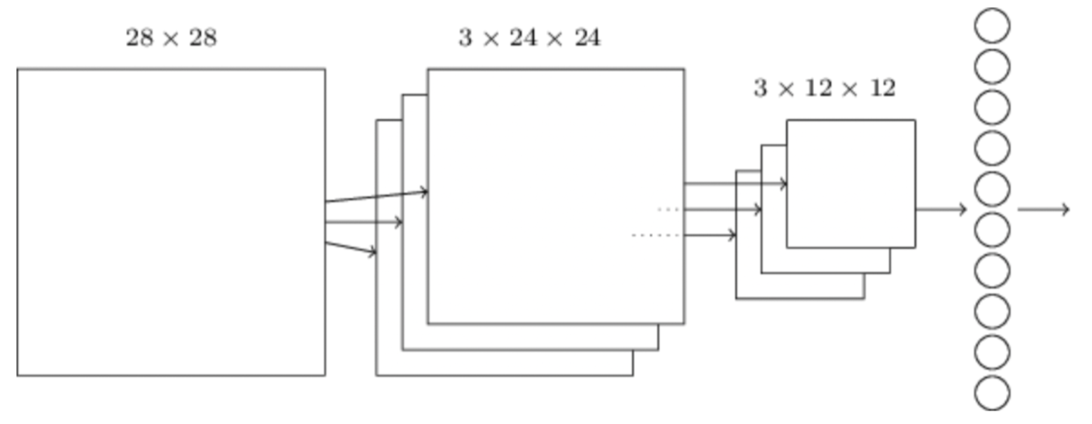
Once the four blocks are done, let's add an adaptive global pooling layer. It collapses each feature map down to a single number by averaging its values.

As I mentioned earlier, in the data section, our region of interest is not a fixed spot in the image since some participants speak louder or later than others. So here we throw away position and keep only the info about how prominent the feature is somewhere in the image.

Flattening the layer

x.view()

We use x.view() to just reshape the adaptive pooling layer's output (256×1×1) into a flat vector. Now the following linear layers can connect to it.

Fully connected layers

nn.Linear() with ReLU + Dropout

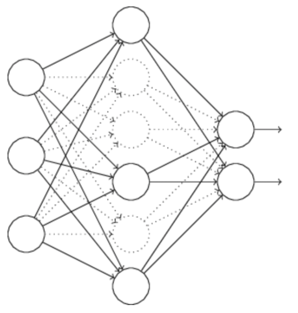
Finally, let's add a classifier tail at the end of NN. This is three classical linear layers that are needed to narrow the output from 256 to 128, then to 64, and finally to 2 (the output layer's size). The last 2 is our two classes (PA and TA) as raw logits.

Between the linear layers, let's add nn.Dropout(0.5). During training, this randomly "deletes" half the neurons (each pass, different ones) in the layer. By this, we simulate the scenario of training many different models (each making its own mistakes and overfitting in its own way) and combine their results at the end to average the effects and hopefully reduce overfitting.

Training

So far, the predictions the model makes are utter trash. That's because the weights and biases are still random. In order to fix them, we need to run training.

Training means repeatedly checking how wrong the model's predictions are, computing the gradient of that error with respect to every weight and bias, and nudging the weights and biases a small step in the negative gradient direction (the direction that makes the error smaller).

Training loop

Let's put together some main pieces of the training loop: a forward pass, loss calculation, backward pass, and weights/biases update. We are also interested in tracking some metrics (loss and accuracy) along the way. All this will be wrapped in a single function called train_epoch().

First, let's put the model into training mode with model.train(). This matters because of two layers in the architecture: BatchNorm and Dropout. In training mode, BatchNorm uses the statistics of the current batch, while Dropout "deletes" half the neurons. In evaluation mode (model.eval()), BatchNorm falls back on running statistics collected during training, and Dropout is turned off.

Then, let's set up three running counters to report the epoch's average performance: total_loss, total_samples, total_correct.

For me, the matter of convenience is to wrap train_loader in tqdm(). I hate silence, and I am a control freak. I need a live bar that shows the progress.

Now, how does the main loop work for each batch of (images, labels):

• First, it resets the gradients before new calculation (optimizer.zero_grad()). Otherwise, we will add new ones on top of the old calculations since PyTorch accumulates gradients on every .backward() call.
• Then it performs a forward pass to get predictions.
• Calculates the loss with CrossEntropyLoss (which is the standard loss function for classification). It expects raw logits because it applies softmax internally.
• Performs backward pass: loss.backward(). Autograd computes the gradient of the loss with respect to every single weight and bias.
• Finally, it updates weights and biases with optimizer.step(). I use Adam because it adapts its step size per parameter instead of using one fixed step size.

It accumulates this batch's loss (total_loss), how many samples we've seen (total_samples), and accuracy (total_correct). Once every batch is done, get the epoch's average loss by dividing total_loss by the number of batches. Divide total_correct by total_samples to get accuracy. Epoch's loss and accuracy are the two values that the training function returns.

Validation loop

Training metrics are important, but we are truly interested in validation metrics - how the model performs on spectrograms it has not seen before. For this, let's build a validation loop called validate_epoch().

The first line is model.eval(). It is like model.train() from the training function, but it switches BatchNorm and Dropout into validation mode.

Let's prepare the same running counters as before: total_loss, total_samples, and total_correct. But this time, let's add two more: empty lists all_predictions and all_labels. We will need them later for the confusion matrix.

The structural difference from the training loop is that the validation loop includes torch.no_grad(). We do not need to update weights and biases, but just check how well the model performs. Apart from this, we use the same forward pass and count the same loss.

The loop for each batch:

• Forward pass
• Loss
• Predictions and true labels get appended to the running lists.

At the end, it performs the same epoch-average math as in the training loop.

This time, the function returns four things: epoch_loss, epoch_acc + lists of all predictions (all_predictions) and all labels (all_labels).

Main training loop

We now have two building blocks: one epoch of training, and one epoch of validation. But neither of them trains the model on its own. Now it is time to combine them together.

Let's first set up a dictionary for the trained_model = {'train_loss': [], 'train_acc': [], 'val_loss': [], 'val_acc': []}. This is where we will store metrics for each training epoch.

Also, let's create two more variables best_val_acc = 0.0 (to remember the best validation accuracy seen so far) and a patience mechanism patience = 10, patience_counter = 0. The last one is for early stopping, which works like this: every epoch that doesn't beat the current best, patience_counter goes up by one. The moment an epoch does beat it, the counter resets back to 0. Once patience_counter reaches patience, training stops. 10 epochs in a row with no improvement is a sign the model has learned what it's going to learn from this data.

For each epoch:

• train_epoch(...) runs one full pass over the training data.
• validate_epoch(...) runs one full pass over the validation data.
• scheduler.step(val_loss). The scheduler here is ReduceLROnPlateau, and it watches val_loss, and if that hasn't improved for patience=5 epochs, it multiplies the learning rate by factor=0.5 (cutting it in half). The logic is that early in training you want big steps to make fast progress. Later in learning, once the model plateaus, big steps cause overshoot, so we need them smaller.

Note that the scheduler's patience=5 is about the learning rate, while the early-stopping patience=10 is about stopping training entirely.

After that: print the epoch's stats, append them to our history dict, and check if val_acc did beat best_val_acc. If yes:

• reset patience_counter to zero,
• write the model weights and biases by checkpoint: torch.save({...});
• save optimizer's internal state, epoch number, val accuracy, and val loss to disk as one .pth file.

If no, patience_counter goes up by one, and we check it against patience. Once we reach the limit, break out of the loop.

My numbers for the training: I set Adam with an initial learning rate = 0.001, a scheduler factor = 0.5, patience = 5. Dropout = 0.5, batch size = 32, early stopping with patience = 10.

Training ran for 17 epochs before stopping. Validation accuracy = 88.16%, validation loss = 0.31.

I decided to stop here and check the results, then go for the second round of training.

Inference

Once the best checkpoint was saved, the next question is whether the model could actually distinguish PA from TA on the spectrograms it had never seen.

I realized that the accuracy on the validation set (88%) was not high enough, but I hoped to obtain more correctly labeled examples (+ those I would have corrected during manual review) to expand the initial dataset for the second round of training.

Single image inference and evaluation

Initially, I began performing inference by processing images one by one. I loaded an image, converted it to RGB format, and applied the same transformations used during validation (because the model is highly sensitive to this). If the input data differs even slightly from the training data, confidence scores can become unreliable.

The output is two logits (as before). I used softmax to raise each score to the power of the exponential and divide by their sum. The result is two non-negative numbers that sum exactly to one. Now the rest is to choose the higher one. It gives both the predicted class and how sure the model is about it (confidence).

Labeling the rest of the dataset

Remember that this project existed only because nobody wanted to sit through thousands of recordings and label them by hand. I labeled 1600 myself to get the model some starting training set - now it was time to label the rest.

First, I loaded the master CSV containing participant number, trial info, image path, audio path, and label (the same file from the data section). I filtered out hand-labeled trials. Then I ran the model over what was left. Two new columns were added to the table: predicted label and confidence. class_names[prediction.item()] converted the index back into the actual string label PA/TA.

This is the part that made the whole approach worth it! Instead of manually labeling the remaining few thousand examples, I ran them all through the model and received the confidence scores. These confidence scores served as a signal indicating exactly what I should focus on during manual review.

Manual review

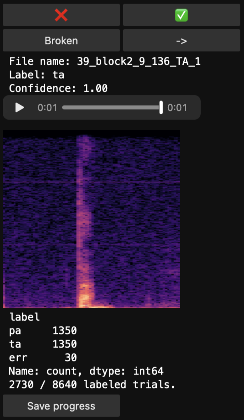
Here, I decided to use the same review widget from before. When the display is updated, the program reads the CSV with the model's predictions and filters out only rows that have predicted labels. Then it takes one random row and displays the sound, its corresponding spectrogram, the predicted label, and the confidence score.

Regarding widgets.Button(), two new buttons were used:

• Correct (copy the predicted label to the "label" column and move on to the next trial)
• Incorrect (write the opposite of the predicted label to the "label" column and move on to the next trial)

The idea was not just checking predictions for the sake of checking, but to use every correction as a new labeled example for the next round of training. I'm glad the time spent on verification didn't go to waste!

Plus, I added a prediction filter based on the desired confidence range (to move from the lower to higher confidence). This allowed me to grow the training dataset by adding the trickiest and most ambiguous sounds with the lowest confidence.

I went through around 1500 predictions until I was too tired and sure that the accuracy wasn't where I wanted it.

The second training round

Combining the corrections with the original 1600 gave me 3213 labeled examples (1538 for PA, 1675 for TA - balanced enough). I used the same 80/20 split as before (reproducible split), which left me with 2570 examples for training and 643 examples for validation. The whole setup and hyperparameters were the same as in the first round.

Training stopped at epoch 17. Validation accuracy = 97.22%, validation loss = 0.12. Such an improvement!

I reviewed the new predictions the same way (widget and confidence logic):

I sorted by confidence and started from the bottom. This led me to roughly 1000 of the lowest-confidence trials. I stopped checking individually past the 89% mark because there was nothing to correct anymore - the model's predictions were correct. I walked a little through the rest 11% of confidence anyway, checking some random trials. I confirmed that the rest of the predictions were correct.

Conclusion

Ultimately, all 8,480 files were labeled and sent to the scientists as a CSV table. These labels were subsequently used in further statistical analysis.

Looking back, I think that what I did was similar to the human-in-the-loop process. I had a small set of manually labeled data. The model predicted the rest, assigning a confidence level to each prediction. I used that confidence level to determine exactly where the results needed to be verified. And the verified results were then immediately used for the next stage of training.

Also, confidence turned out to be useful for one more thing, which is catching actual errors in the data, since all these broken/silent trials were in the low-confidence group. Instead of searching for them throughout the whole dataset, I was able to identify and clean them all relatively easily, in two passes (30 from the manual labeling + 36 during the manual review = 66 trials in total).

Funny side note: some of the PA and TA sounds were very hard to tell apart, even for me (a person who has a musical background). I even asked a few colleagues to listen, but none of us agreed with each other. So apparently, this model does its job more consistently than a human ear.